By John M. Steinberg & Grace E. Bello
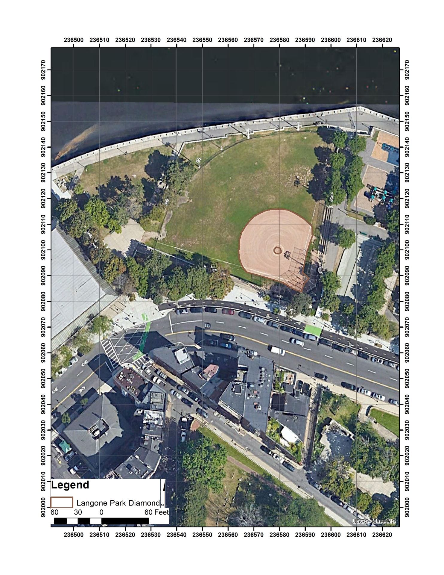
View of softball diamond at Langone Park. The infield and pitcher’s mound is outlined in brown, which helps to orient the following geophysical images.
As we said in our previous post, the City Archaeologist, Joe Bagley asked us at the Fiske Center if we could conduct a geophysical survey over the area of Langone Park that, 100 years ago, had a tank which ruptured and caused The Great Molasses Flood of 1919. This is in preparation for Tuesday January 15th, 2019—the 100th anniversary of the disaster.

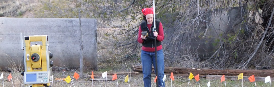
Grace Bello beginning to set up the geophysical grid by placing PVC flags along the first base line.
For our archaeological geophysical survey, we used two common techniques: ground penetrating radar (GPR) and electromagnetic (EM) conductivity. The area was first prepared for the survey by placing out a grid of PVC flags. Because the grid was oriented to the softball diamond, the locations of each of the corner flags (and many of the intermediate flags) were recorded with a survey grade GPS.

John Steinberg walking along the third base line with the CMD-Mini.
First, John used the CMD-MiniExplorer conductivity meter, which requires the operator to walk across the target area holding the unit just above the ground. These transects are then combined to create a conductivity map of the subsurface. The CMD-Mini creates a data set with two components at three different “depths.” The different depths are from the three different receivers in the orange tube at various distances from the single transmitter. The farther apart the receiver from the transmitter, the “deeper” the reading (1 is the closest, 3 is the farthest and thus deepest). The two components are complex. The Quadrature component, usually called bulk conductivity (Con) represents the apparent conductivity of the volume of earth under the unit and is measured in milli-Siemens per meter (mS/m). Good conductors (e.g., salty wet earth) have high conductivity, while poor conductors (e.g., rocks) have low conductivity. The in-phase component (IP) is usually expressed in parts per thousand (ppt) and is very sensitive to buried metal. Thus, we have a total of six different maps from the CMD-Mini: Con1 & IP1, Con2 & IP2, and Con3 & IP3.
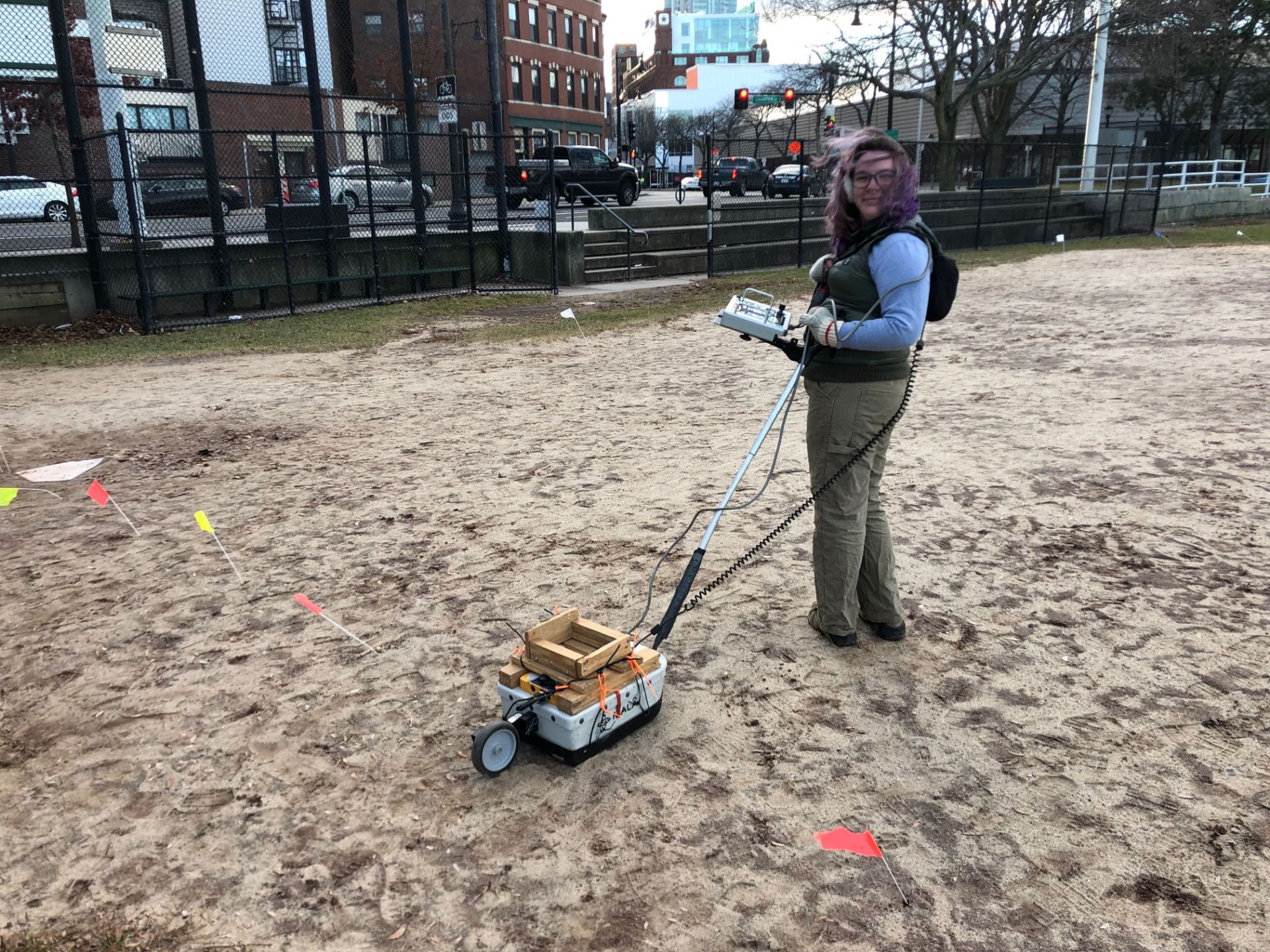
Grace Bello with the Malå GPR unit.
Second, Grace and John walked back and forth dragging the Malå GPR unit with a 500 MHz antenna. The GPR unit sends out microwaves and if there is a change in soil moisture (or some other similar property) some of the microwave energy will be reflected back up to the GPR unit, which also has a receiver. The GPR unit then, like the CMD, collects data along transects which produce a data stream called a radargram. Multiple transects are combined and then sliced at different depths, which allows us to create a series of maps that depict some of the aspects of the changes in the subsurface at different depths. We created 25 different slices, but only present two below.
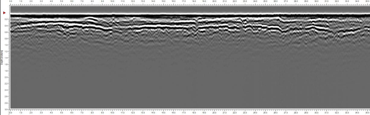
Example radargram from the transect 5 m (16.5 ft) north of the third base line.
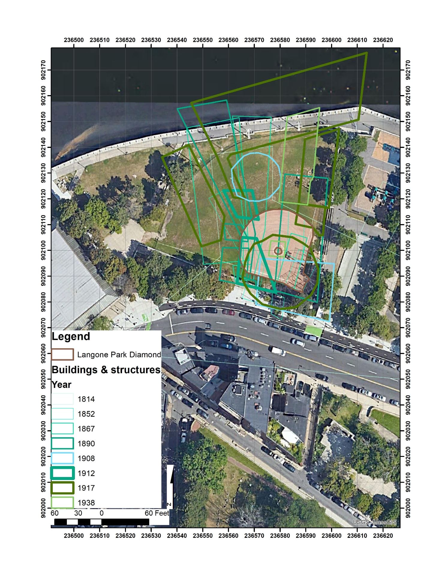
Outlines of all the structures from the maps described in our previous blog post
In our recent blog post, we describe the georeferencing of various historic maps of Langone park. When all of the various structures depicted on these maps are combined, you can get a sense of just how complex this lot is. Many of the structures may be the same structure, but with slightly different locations provided by different maps, and we do not know how accurate any of them are. In this case, we have been asked to identify one of the last structures on the lot. Generally, the construction of later structures compromises or destroys the earlier structures. Thus, our most likely potential target is an area where there is a broad, consistent absence of distinct structures. Furthermore, given the hasty construction of the tank, any remements are probably shallow. This approach is in stark contrast to our usual method—where we are trying to identify remnants of the earliest structures.

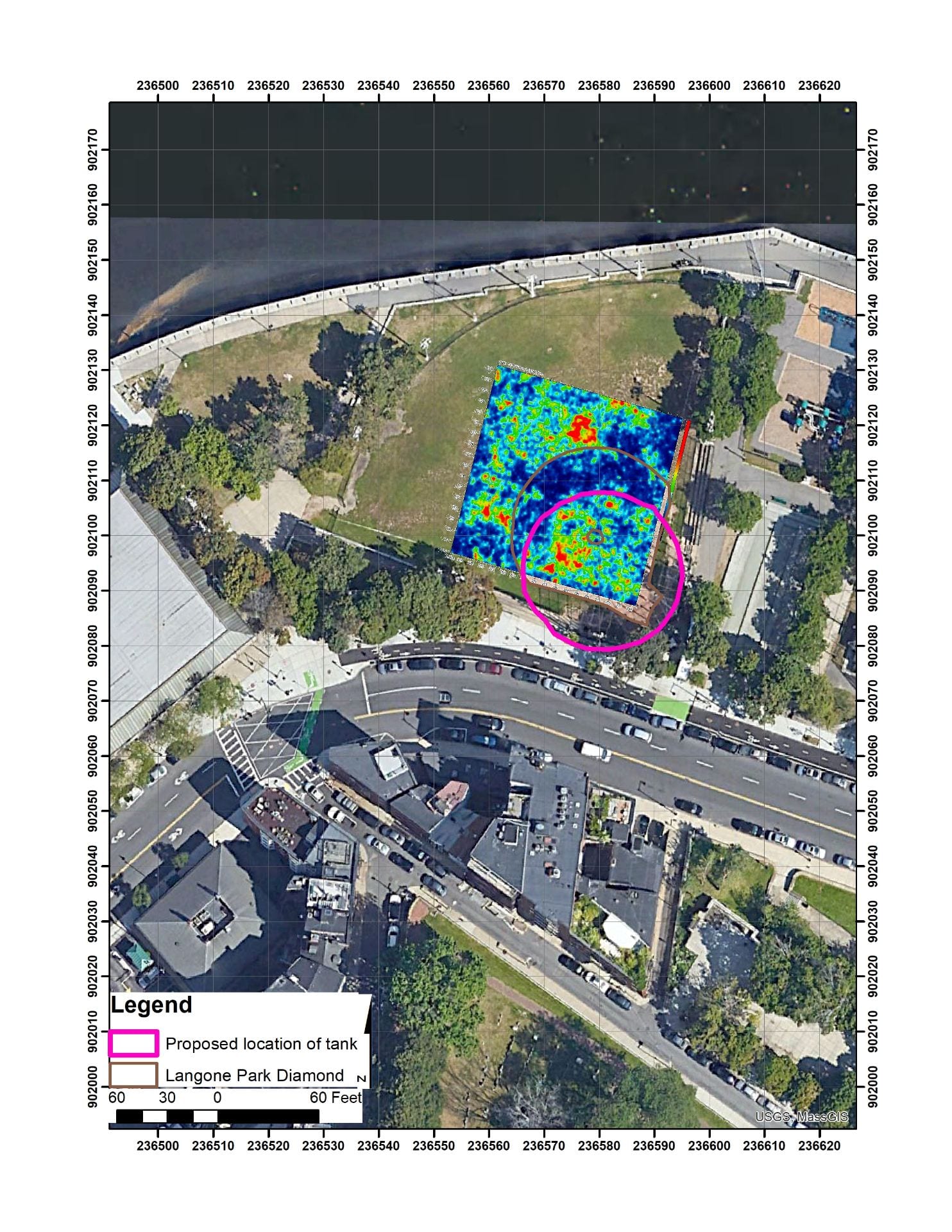
GPR slice 50 cm (about 20 in) below the ground surface.

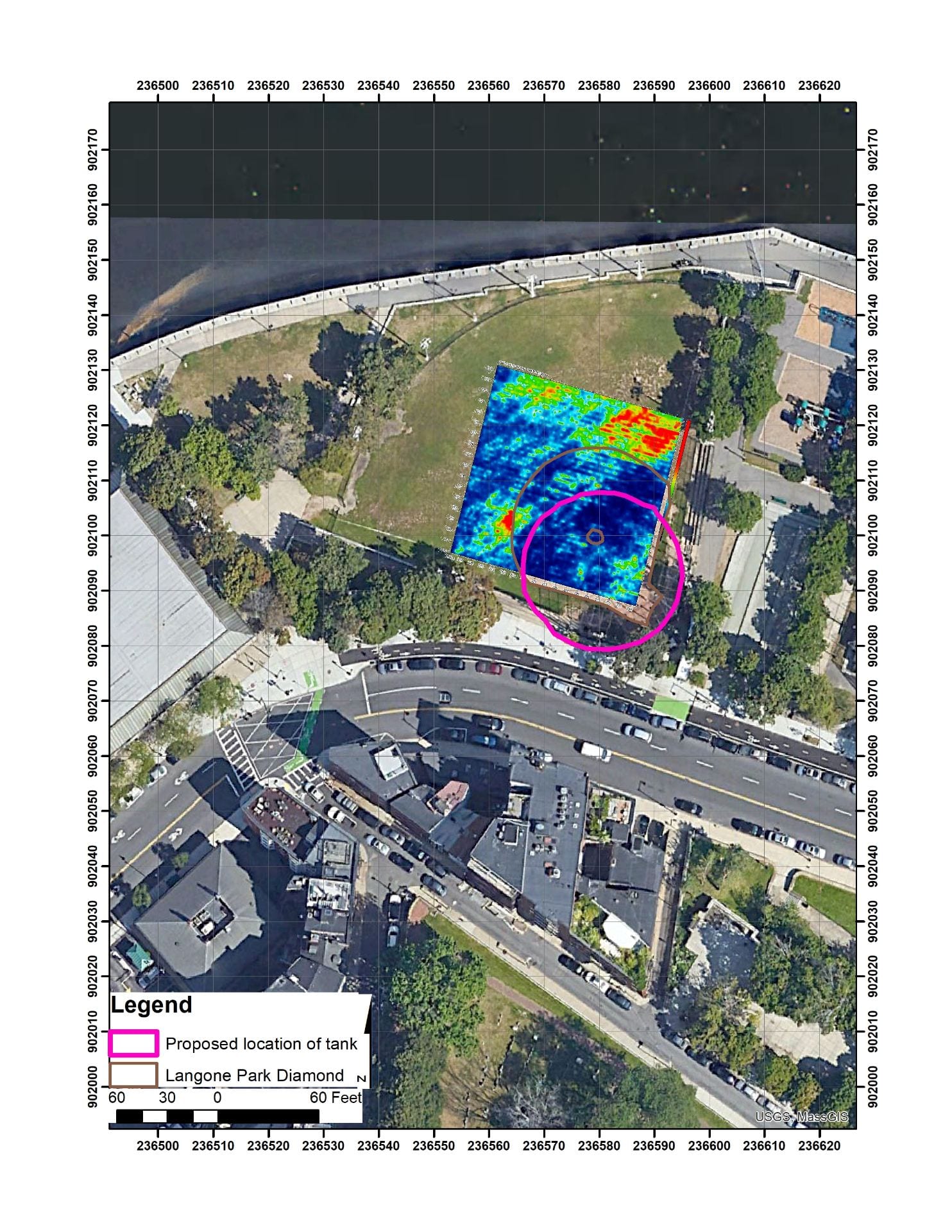
GPR slice 150 cm (about 60 in) below the ground surface.
Starting with the GPR results, there is a distinct hard reflector 50 cm below the ground surface (bgs). This hard reflector is circled in pink. This infield hard reflector is distinct from the outer edge of the infield (marked in brown). This hard reflector is potentially caused by the remnants of the tank in question. That being said, we want to be a little careful, because this hard reflector is almost the same as the grass infield area from when this was a little league diamond. However, this slice is a little too deep to show that contrast. Furthermore, the wide dirt path from the mound to home plate is not visible in this slice. Both of these lines of evidence suggest that this hard reflector is a result of current or recent landscaping. The deepest GPR slices do not seem to show remnants the tank but instead show some of the potential dock and landfill boundaries, just to the north of first base. Interestingly, this dominant southeast angle does not reflect any of the structures or orientations seen in our georeferenced maps.

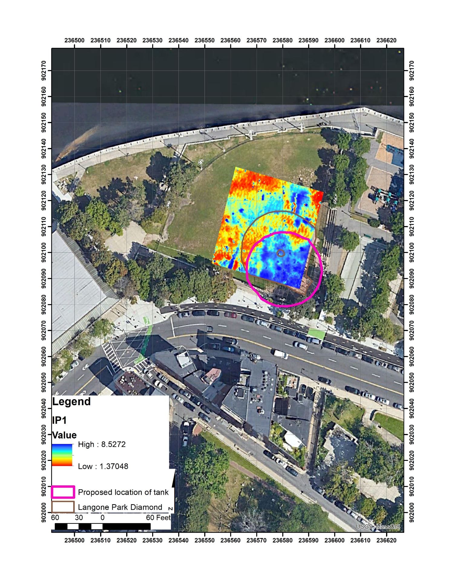
In-phase for the most shallow CMD-Mini readings (IP1). The potential tank location is in pink.
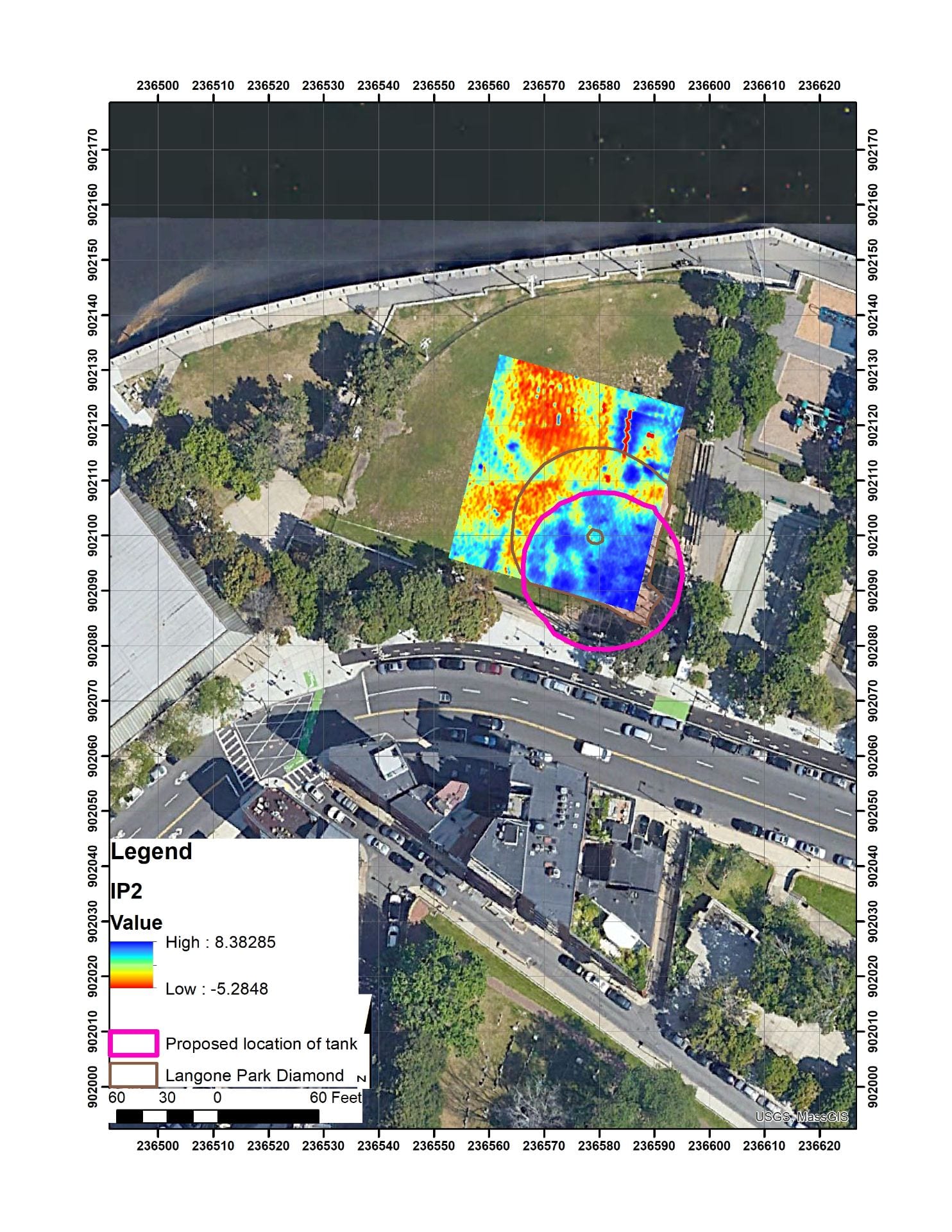
In-phase for the middle CMD-Mini readings (IP2).
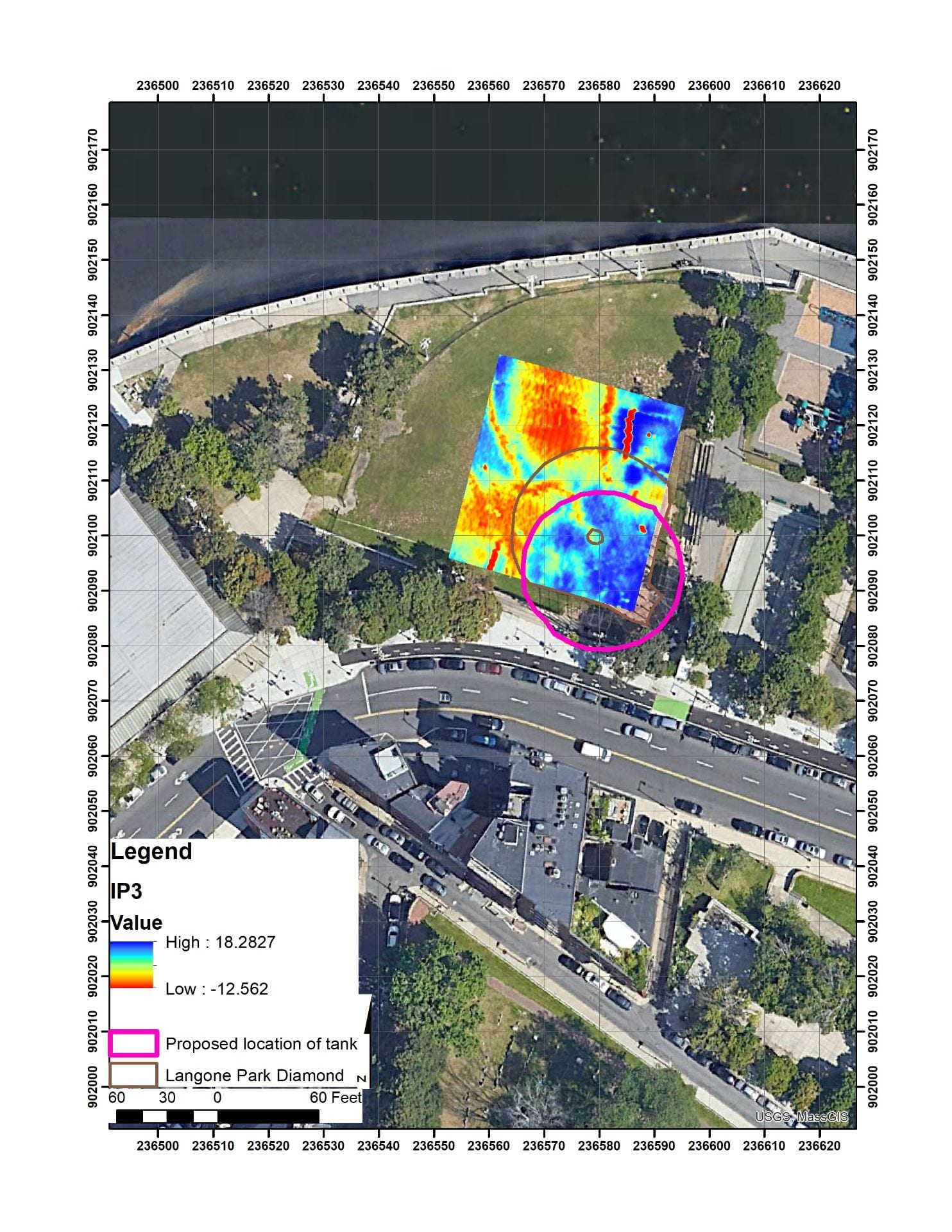
The CMD-Mini yields much more complex results that correspond to many of the structures outlined in the georeferenced maps. Starting with the IP components, IP1 shows a blue (high IP) area in the infield that corresponds to the area identified in the GPR (again circled in pink). Just north of the first base line, in right field, is a rectangular blue area that has the same general dimensions and orientation as the structure seen in the 1917 map, just north of the tank in question. That structure has an add on (in brown) that curves along the curve of the tank that touches 1st base. The potential tank area is more distinct in the deeper components (IP2 & IP3), while the building in right field is less distinct.
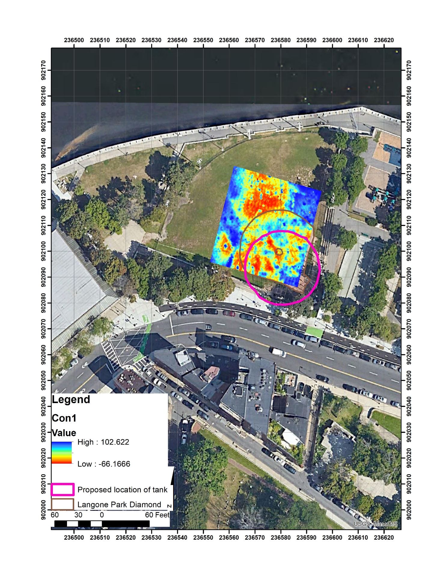
Conductivity for the most shallow CMD-Mini Readings (Con1).
The bulk conductivity component of the data from the CMD-Mini is much more complex, but all three sensor-transmitter distances show the same basic map.

In-phase for the deepest CMD-Mini readings (IP3). The potential tank location is in pink

Conductivity for the middle CMD-Mini Readings (Con2).

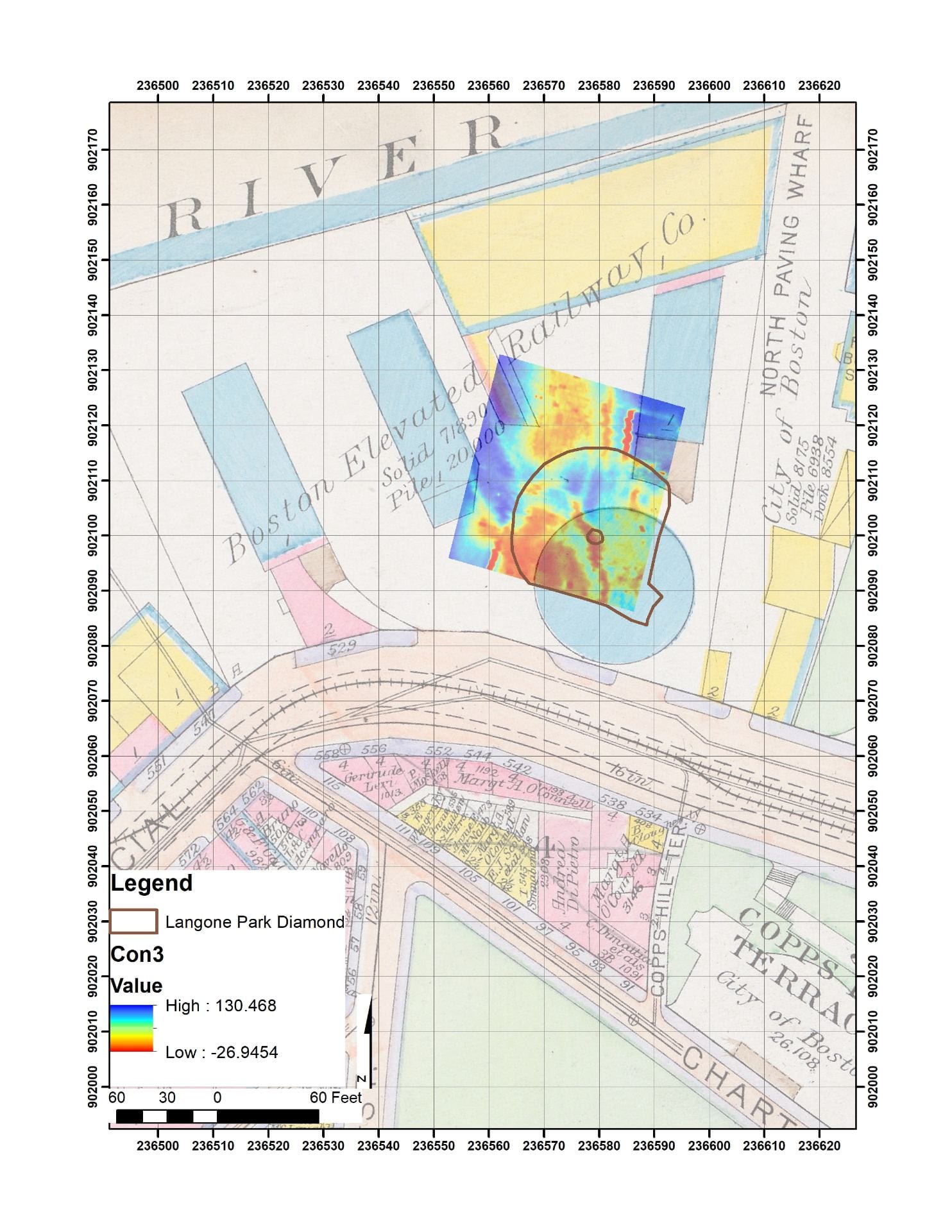
The Slatter 1852 Map with Con3 superimposed.
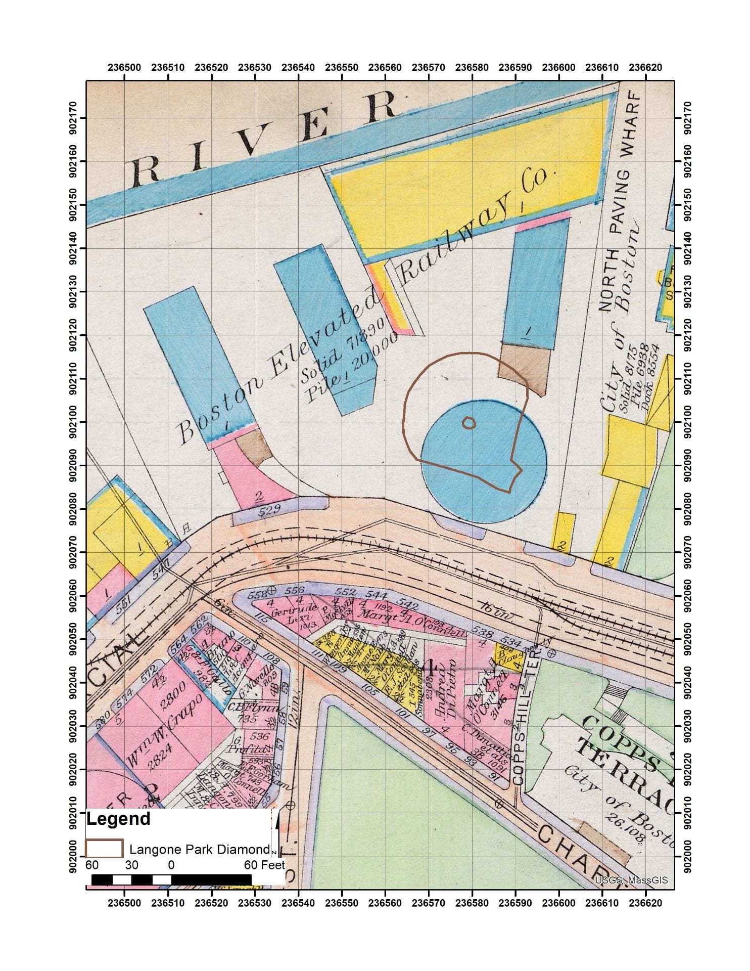
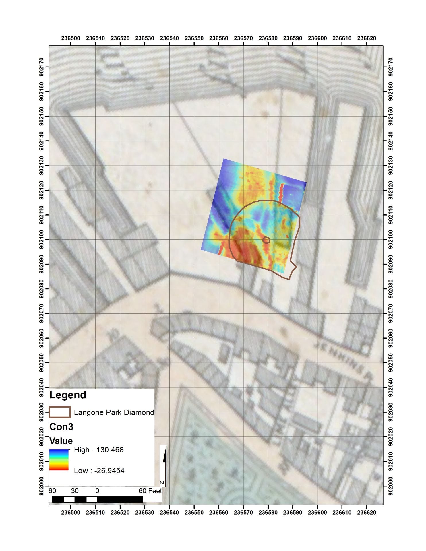
The Bromley 1917 map with Con3 superimposed.
Unlike the IP, the Con does not hint at the tank location, there are three high (blue) conductivity areas that seem to correspond to the distribution and orientation of structures in some of the georeferenced maps. The blue area in left center field matches quite closely with the angled structure drawn in the 1852 Slatter map. Some of the low conductivity lines (which could be lines of rocks) correspond to lines drawn in that 1852 map. Once a property orientation is established, it tends to persist. Thus, it is not surprising that the geophysics can correspond to more than one map. Specifically, the three blue areas in the outfield roughly correspond to the three drawn structures abutting the tank in question depicted in the 1917 Bromley map.

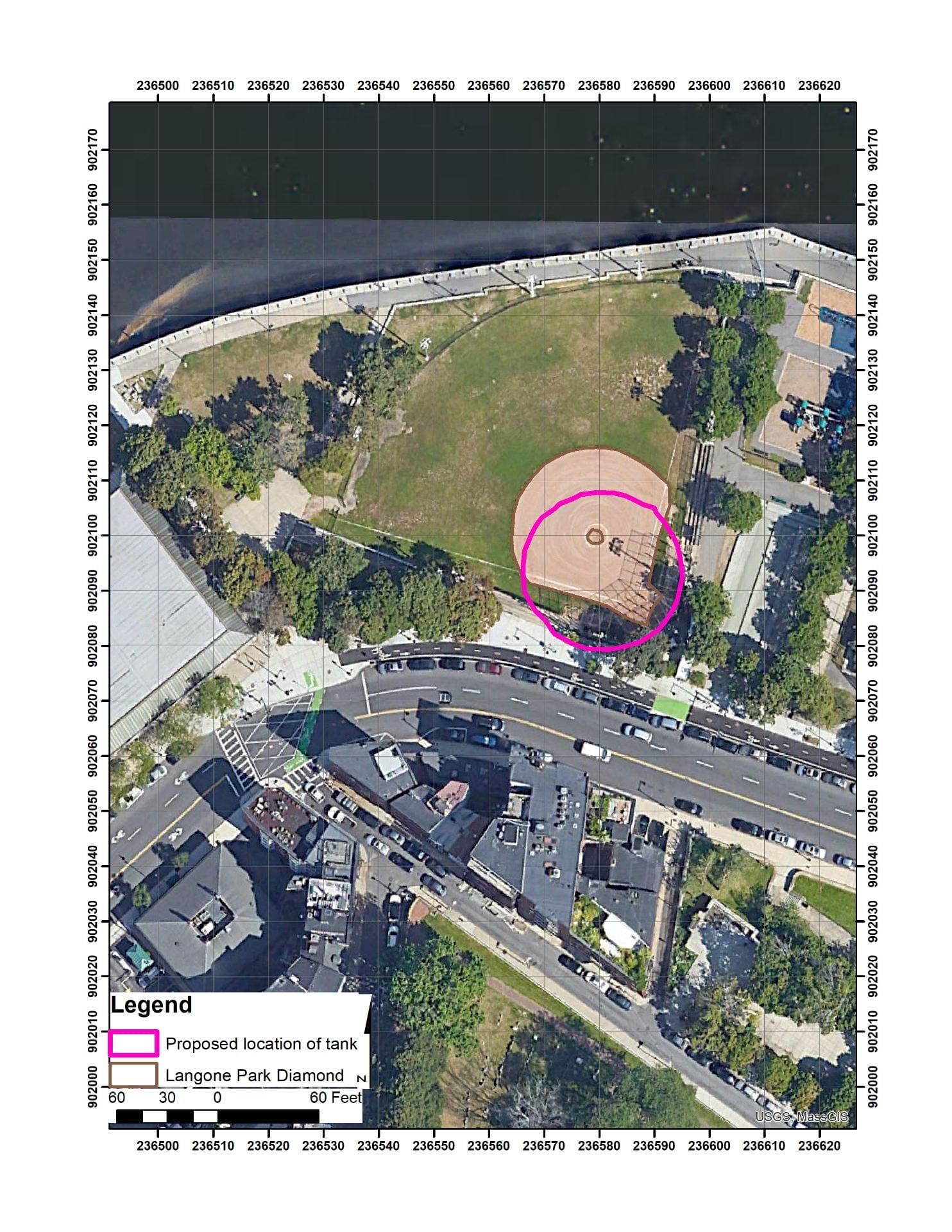
Proposed location of tank superimposed on air photo.
While in both the 1852 and 1917 maps the correspondences with geophysical readings and drawn structures are not exact, they are well within the range of accuracy that we usually see with these kinds of maps.
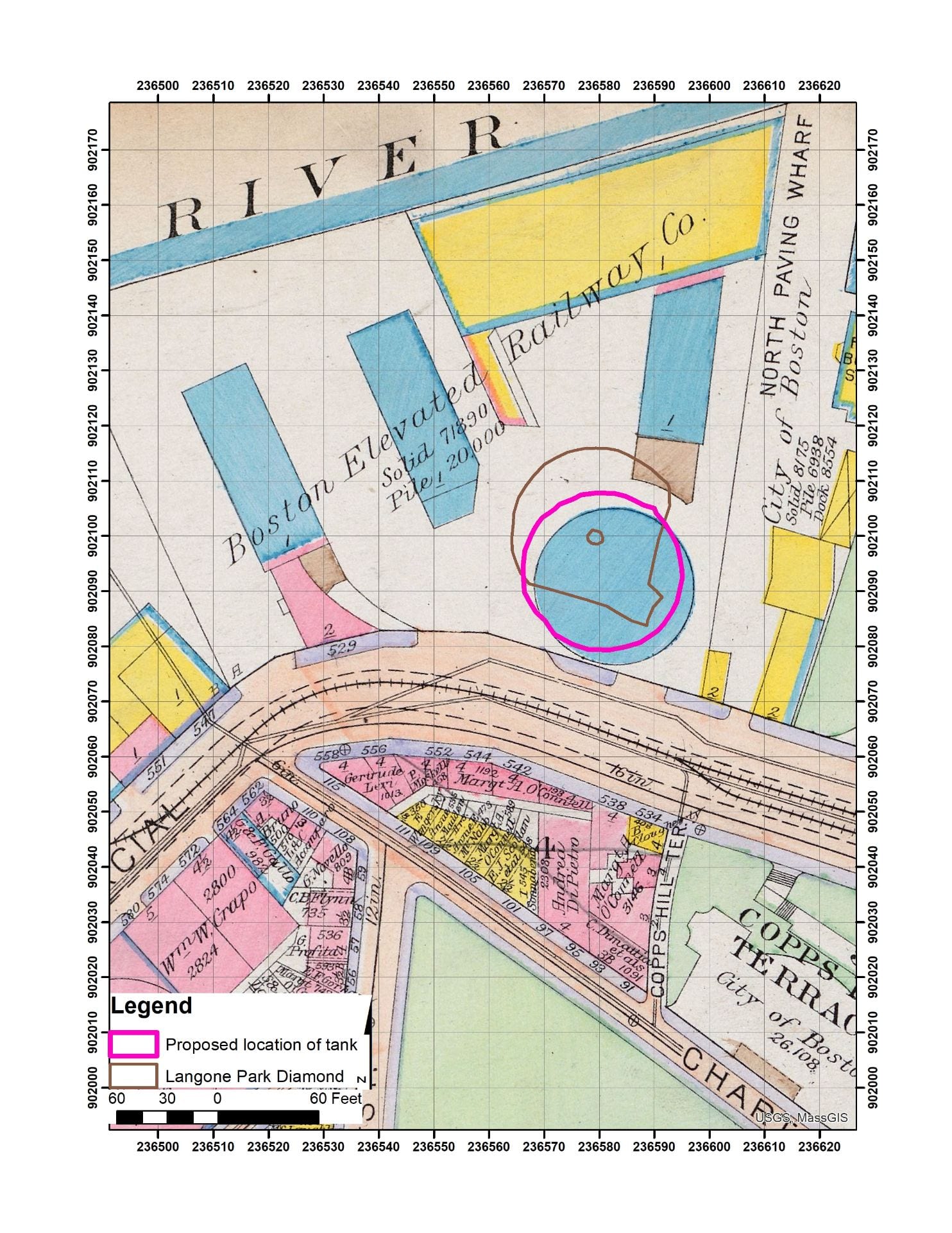
When all of our data is combined (the georeferenced maps, the GPR and the Electromagnetic Conductivity) and tried to make fit, our best guess as to the specific location of the remnants of the tank that caused the Great Molasses Flood, is 3 meters northwest of the location drawn in the 1917 Bromley map—at least by our georeferencing of that map. Obviously, we would need to excavate this dynamic and interesting area to begin to refine the location further, but the geophysical results suggest that the 1917 map is generally accurate. There is no evidence of a consistent bias in the locations of structures as compared to the geophysics, so as georeferenced, the 1917 map is accurate to better than 5 m (16 ft). As always, more research is necessary.

The 1917 Broomly map with the proposed actual location of the tank in pink.